Practical 1

Data manipulation

This exercise will practice several of the ‘essential data manipulation’ tasks covered during the lecture, including selecting, sorting, merging, grouping, and summarising.

The MovieLens dataset

We’ll be using a subsample of the MovieLens dataset (available at this page). This dataset contains 20 million ratings applied to 62,000 films from 162,000 users. Fortunately, the random sample we’re using is slightly smaller: 100,000 ratings for 9,000 films.

First, load the tidyverse package:

library(tidyverse)

Import and merge

Download movies.csv and ratings.csv and import both datasets into R using read_csv. Store as two data frames.

movies <- read_csv("../data/movies.csv")
ratings <- read_csv("../data/ratings.csv")

Tip: Portable paths with the here package

You can use the here package to construct portable file paths (i.e., paths that work across machines). Once you’ve created an RStudio project:

library(here)

here() starts at /Users/ewan/Sync/Work/Projects/Active/Introduction to R (HDR UK March 2026)/website

movies <- read_csv(here("data", "movies.csv"))

Rows: 9742 Columns: 3

── Column specification ────────────────────────────────────────────────────────
Delimiter: ","
chr (2): title, genres
dbl (1): movieId

ℹ Use `spec()` to retrieve the full column specification for this data.
ℹ Specify the column types or set `show_col_types = FALSE` to quiet this message.

ratings <- read_csv(here("data", "ratings.csv"))

Rows: 100836 Columns: 4
── Column specification ────────────────────────────────────────────────────────
Delimiter: ","
dbl (4): userId, movieId, rating, timestamp

ℹ Use `spec()` to retrieve the full column specification for this data.
ℹ Specify the column types or set `show_col_types = FALSE` to quiet this message.

This assumes movies.csv and ratings.csv are stored in a folder called data, located in the root of your project.

Merge the two data frames (movies, ratings) to create a single data frame with 100,836 rows and 6 columns.

Solution

dat <- ratings |>
    inner_join(movies)

Joining with `by = join_by(movieId)`

Bonus questions:

What’s the difference between full_join and inner_join in this instance?
Which column was used to merge the two data frames? How could you specify this yourself?

Solution

dat <- ratings |>
    inner_join(movies, by = "movieId")

Summarise

Calculate the mean rating per film.

Hint: You’ll need to use group_by and summarise.

Solution

av <-
  dat |>
  group_by(title) |>
  summarise(mean_rating = mean(rating))

What is the range of average scores?

Solution

range(av$mean_rating)

[1] 0.5 5.0

How many films share the top average rating?

Solution

av |>
    filter(mean_rating == max(mean_rating)) |>
    nrow()

[1] 296

Creating new columns

Use the below code to create a new column containing the year each film was released.

av <- av |>
    mutate(year = str_extract(title, "[0-9]{4}.$"),
           year = parse_number(year)) |>
    drop_na(year)

Bonus questions:

What’s going on here? What does [0-9]{4}.$ represent?
Why have we used a drop_na statement?

Calculate the average rating per year. Store the result in a new data frame, sorted by year (earliest to latest).

Solution

per_year <- av |>
    group_by(year) |>
    summarise(year_mean = mean(mean_rating)) |>
    arrange(year)

Plotting

(Optional) Plot the average rating (y-axis) by year (x-axis).

We haven’t covered plotting yet, but it seemed natural that we’d want to plot something at this stage. So for now, try (copy-and-paste) either of the below options (you may need to adjust the variable names, depending on what you chose above):

Using base R

plot(per_year$year, per_year$year_mean)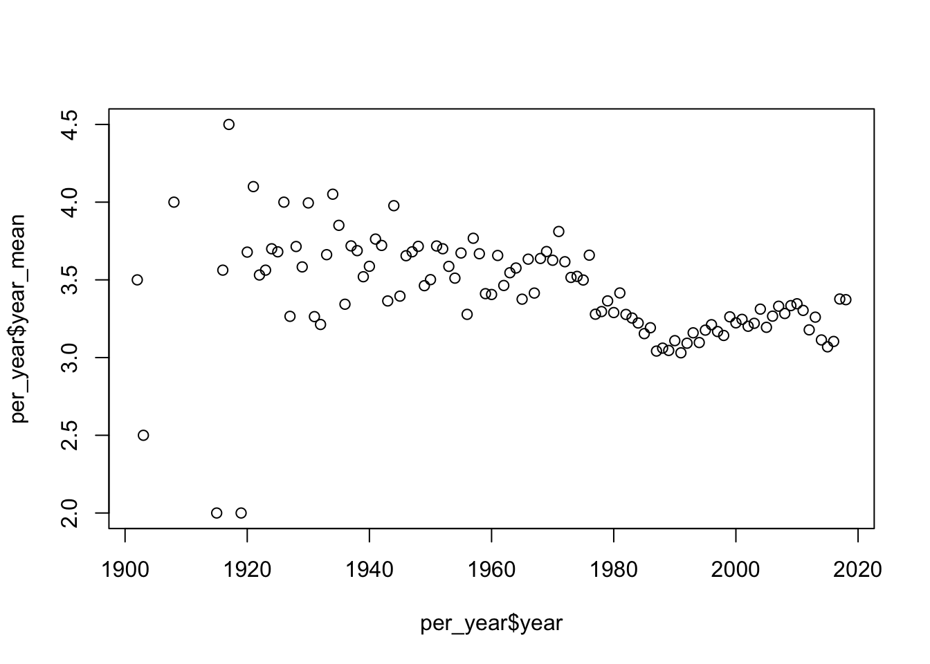

Using ggplot2

per_year |>
  ggplot() +
  aes(x = year,
      y = year_mean) +
  geom_point() +
  geom_smooth()

`geom_smooth()` using method = 'loess' and formula = 'y ~ x'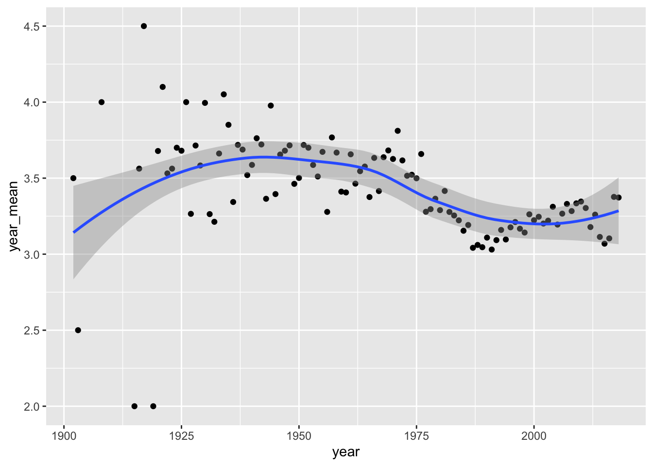

Calculate the correlation between year and rating.

How would you characterise the trend in movie ratings over time?

Solution

cor(per_year$year_mean, per_year$year)

[1] -0.3494103

Calculate the average rating per genre (optional).

You’ll need to split the genre column, reshape, and then recalculate the average grouped score.

Solution

# Separate the 'genre' column by splitting on "|".
dat <- dat |>
    separate(genres,
             sep = "\\|",
             into = paste0("genre", 1:20),
             fill = "right") |>
    select(rating, starts_with("genre"))

# Reshape the data into 'LONG' format
dat |>
  pivot_longer(-rating, values_to = "genre") |>
  group_by(genre) |>
  summarise(mean_rating = mean(rating)) |>
  arrange(desc(mean_rating))

# A tibble: 21 × 2
   genre              mean_rating
   <chr>                    <dbl>
 1 Film-Noir                 3.92
 2 War                       3.81
 3 Documentary               3.80
 4 Crime                     3.66
 5 Drama                     3.66
 6 Mystery                   3.63
 7 Animation                 3.63
 8 IMAX                      3.62
 9 Western                   3.58
10 Musical                   3.56
11 Adventure                 3.51
12 Romance                   3.51
13 <NA>                      3.50
14 Thriller                  3.49
15 Fantasy                   3.49
16 (no genres listed)        3.49
17 Sci-Fi                    3.46
18 Action                    3.45
19 Children                  3.41
20 Comedy                    3.38
21 Horror                    3.26

Going further with MovieLens

This section is optional

We won’t have time to go through this exercise, but I’ve included it here in case you want more practice in your own time.

In this section, we’re interested in movie grossings – how much money did each film take at the box office? Do higher-rated films tend to make more money? What rating should a film have, to maximise the box office takings?

We’ll be using a couple of more advanced techniques:

Scraping data from a website;
Merging and data cleaning.

The MovieLens dataset doesn’t include information on grossings, but we can find this information at https://www.boxofficemojo.com/chart/top_lifetime_gross/.

Use the rvest package to scrape information from this page for the top 1000 films. You should store this information in a data frame with four columns: rank, title, lifetime_gross, year.

library(rvest)


Attaching package: 'rvest'

The following object is masked from 'package:readr':

    guess_encoding

# Create a vector containing the required URLs
url <- "https://www.boxofficemojo.com/chart/top_lifetime_gross"
offsets <- seq(0, 800, 200)
all_pages <- str_glue("{url}/?offset={offsets}")

# For each page, scape the HTML and extract the table

# Using a loop:
tables <- list()
for (i in seq_along(all_pages)) {
  cat(paste("Extracting page:", all_pages[i], "\n"))
  tables[[i]] <- html_table(read_html(all_pages[i]))
}

# Using map:
tables <- map(all_pages, \(p) html_table(read_html(p)))

The read_page and html_table functions will extract the table from a single page, but we’re interested in the top grossing 1000 films, so we’ll need to access multiple pages.

To do this, we need to figure out the URL format:

For the first page, it’s https://www.boxofficemojo.com/chart/top_lifetime_gross/
For the second page, it’s https://www.boxofficemojo.com/chart/top_lifetime_gross/?offset=200
For the third page, it’s https://www.boxofficemojo.com/chart/top_lifetime_gross/?offset=400

So, subsequent pages are specified via the offset argument in the URL. Therefore, we can create a vector containing all required pages and scape the table from each page.

You should now have a list of five data frames. Combine these into a single data frame.

Solution

# Before combining, note that the 'Rank' column is inconsistently recorded. In tables 1-4, 'Rank' is stored as an integer. In the last table it is a character. We need to fix this, otherwise it'll cause problems later:

tables[[5]][[1]]$Rank <- parse_number(tables[[5]][[1]]$Rank)

# There are several ways to combine these data frames.

# Option 1: You could loop through the list of tables and `bind_rows` each one:
# (This is not a great idea).
combined <- tables[[1]][[1]]
for (i in tables[2:5]) {
  combined <- bind_rows(combined, i[[1]])
}

# Option 2: You could use 'reduce' from the purrr package:
combined <- reduce(tables, bind_rows)

Check that your combined dataset has 1000 rows and 4 columns.

Rename the column names and convert the Lifetime Gross column to a numeric type.

Solution

grossing <- combined |>
  janitor::clean_names() |>
  mutate(lifetime_gross = parse_number(lifetime_gross))

Merge this data frame with the ‘mean move ratings’ data frame we generated above (av).

Of the 1000 films in the ‘highest grossing’ data, for how many do we have a corresponding rating for?

both <- grossing |>
  mutate(title = str_glue("{title} ({year})")) |>
  full_join(av)

Joining with `by = join_by(title, year)`

table(!is.na(both$lifetime_gross) & !is.na(both$mean_rating))


FALSE  TRUE 
 9451   628

The first challenge here is that, in MovieLens, the title includes the year:

’71 (2014)

Whereas grossing does not:

Star Wars: Episode VII - The Force Awakens

So, for the formats to match, we need to either remove or add the year. Seeing as we have the year column available in grossing, we can use that.

A second challenge is the difference in how “The…” is handled. In grossing it is before the movie name (e.g., “The Lion King”):

grossing |> filter(str_detect(title, "The"))

# A tibble: 229 × 4
    rank title                                         lifetime_gross  year
   <dbl> <chr>                                                  <dbl> <int>
 1     1 Star Wars: Episode VII - The Force Awakens         936662225  2015
 2     7 Avatar: The Way of Water                           688459501  2022
 3    14 The Avengers                                       623357910  2012
 4    15 Star Wars: Episode VIII - The Last Jedi            620181382  2017
 5    17 The Super Mario Bros. Movie                        574934330  2023
 6    18 The Lion King                                      543638043  2019
 7    19 The Dark Knight                                    534987076  2008
 8    21 Star Wars: Episode IX - The Rise of Skywalker      515202542  2019
 9    23 Star Wars: Episode I - The Phantom Menace          487576624  1999
10    31 The Dark Knight Rises                              448149584  2012
# ℹ 219 more rows

Whereas in the ratings data it is after:

av |> filter(str_detect(title, "The"))

# A tibble: 2,244 × 3
   title                                                 mean_rating  year
   <chr>                                                       <dbl> <dbl>
 1 'Hellboy': The Seeds of Creation (2004)                      4     2004
 2 'Til There Was You (1997)                                    4     1997
 3 'burbs, The (1989)                                           3.18  1989
 4 10th Kingdom, The (2000)                                     2.75  2000
 5 10th Victim, The (La decima vittima) (1965)                  4     1965
 6 11th Hour, The (2007)                                        4     2007
 7 13th Warrior, The (1999)                                     2.90  1999
 8 2 Fast 2 Furious (Fast and the Furious 2, The) (2003)        2.61  2003
 9 2010: The Year We Make Contact (1984)                        3.59  1984
10 39 Steps, The (1935)                                         4.05  1935
# ℹ 2,234 more rows

So, we’ll miss many movies with “The” in the title. If you like, have a go at fixing this. (I haven’t provided code for this, yet).

Using any method you like, answer the two questions below:

Do higher rated films make more money?
What rating should a film have, to maximise the box office takings? What other factors should you consider here?

Solution

# The below code is just one way of answering this question -- many other
# solutions are possible.

# First, let's select films for which we have grossing and rating data:

both <- drop_na(both)

# Second, I'm going to scale the units to "millions of $" so they're easier to
# work with.

both$millions <- both$lifetime_gross / 1e6

summary(both$millions)

   Min. 1st Qu.  Median    Mean 3rd Qu.    Max. 
  87.07  107.29  136.92  170.99  200.08  936.66

hist(both$millions)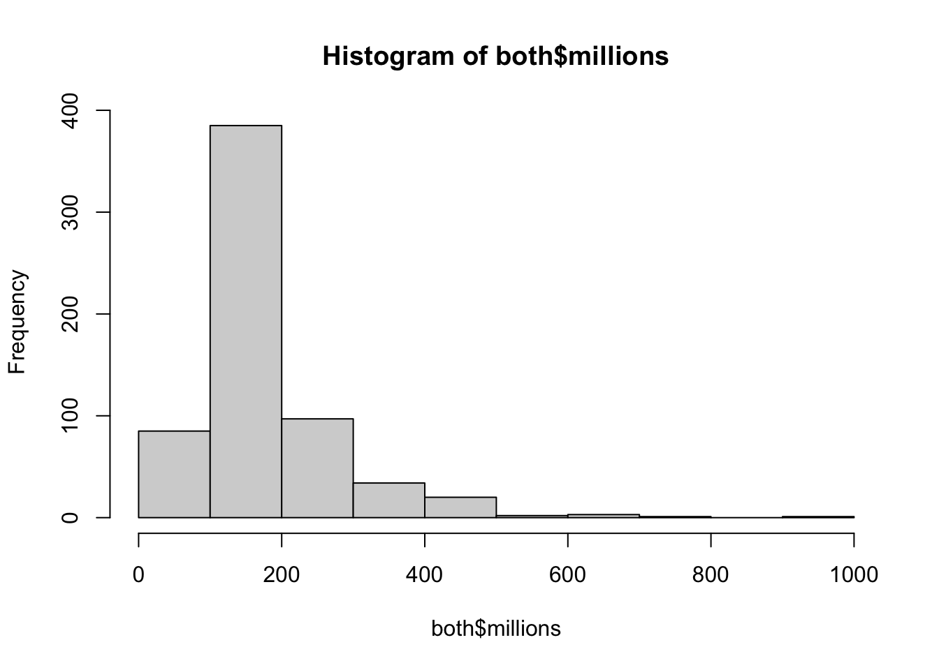

# There are a few films (e.g., "Star Wars: Episode VII" and "Avatar") that
# had were very high grossing. They're not outliers, but I'm going to remove
# them for now.

tail(arrange(both, millions))

# A tibble: 6 × 6
   rank title                          lifetime_gross  year mean_rating millions
  <dbl> <glue>                                  <dbl> <dbl>       <dbl>    <dbl>
1    20 Rogue One: A Star Wars Story …      533539991  2016        3.93     534.
2    16 Incredibles 2 (2018)                608581744  2018        3        609.
3    10 Jurassic World (2015)               653406625  2015        3.26     653.
4     9 Titanic (1997)                      674354882  1997        3.41     674.
5     4 Avatar (2009)                       785221649  2009        3.60     785.
6     1 Star Wars: Episode VII - The …      936662225  2015        3.85     937.

both <- both |> filter(millions < 600)

# We can now plot the linear relationship between ratings and grossings:

both |>
  ggplot() +
  aes(x = mean_rating,
      y = log(lifetime_gross)) +
  geom_point(alpha = 0.5) +
  geom_smooth(method = "lm")

`geom_smooth()` using formula = 'y ~ x'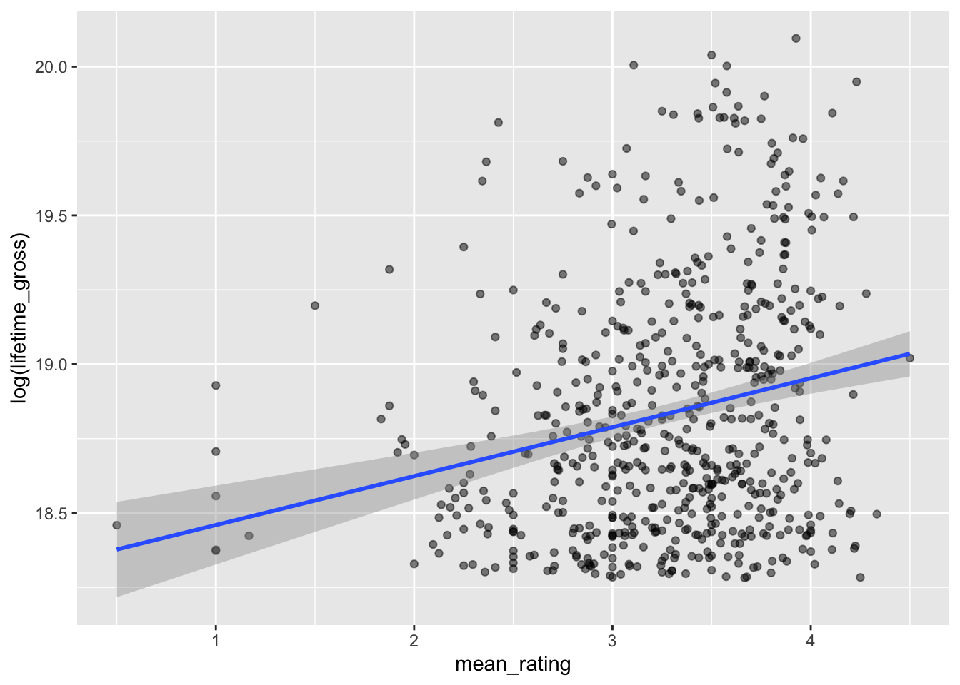

# It's quite likely that the relationship is non-linear. Therefore, let's use
# the 'marginaleffects' package to plot predictions from a linear model with
# a quadratic term.

library(marginaleffects)

# Linear model, quadratic slope
fit_lm <- lm(millions ~ mean_rating + I(mean_rating^2),
             data = both)
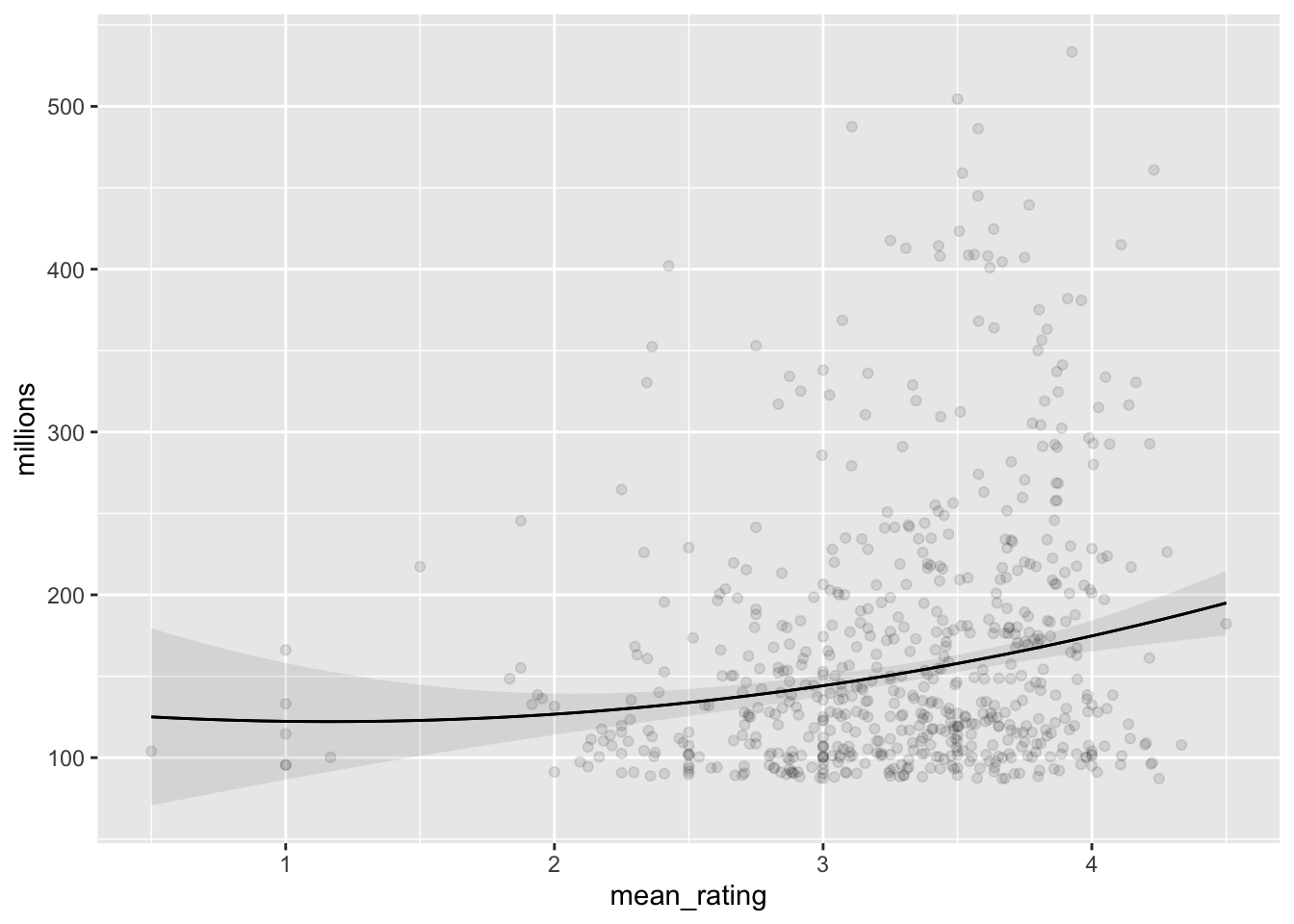
plot_predictions(fit_lm, "mean_rating", points = 0.2)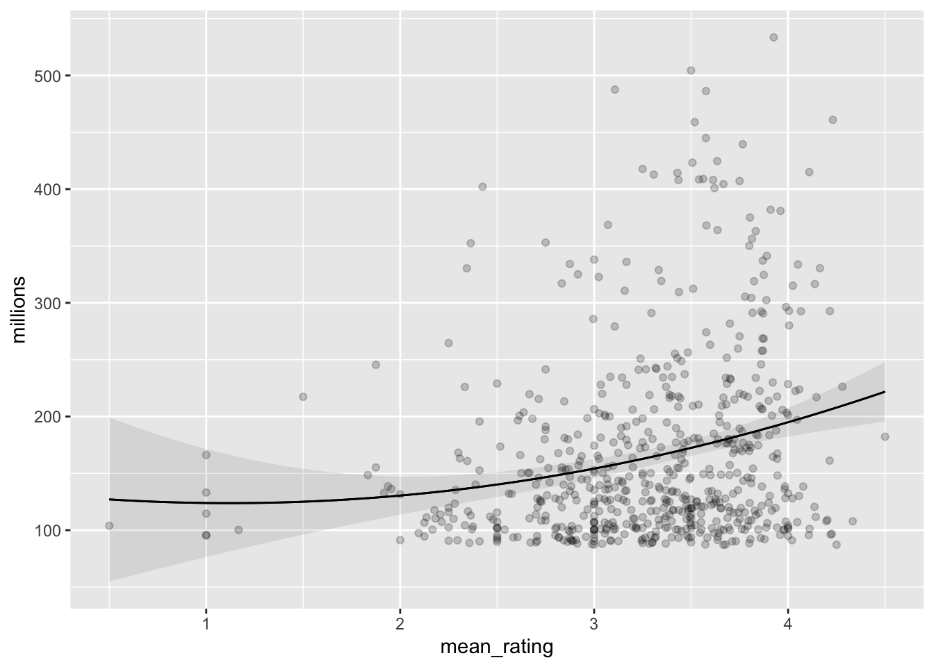

# Robust linear model, quadratic slope
fit_rlm <- MASS::rlm(millions ~ mean_rating + I(mean_rating^2),
                     data = both)
plot_predictions(fit_rlm, "mean_rating", points = 0.1)