πŸ₯ Session 2 (β€œIntermediate”)


This session will begin by introducing key concepts in R programming, including functions, iteration, and control flow. You’ll learn how to create your own functions to automate repetitive tasks and streamline your workflows. We’ll also explore iteration techniques, discussing R-specific approaches to handling repeated operations efficiently.

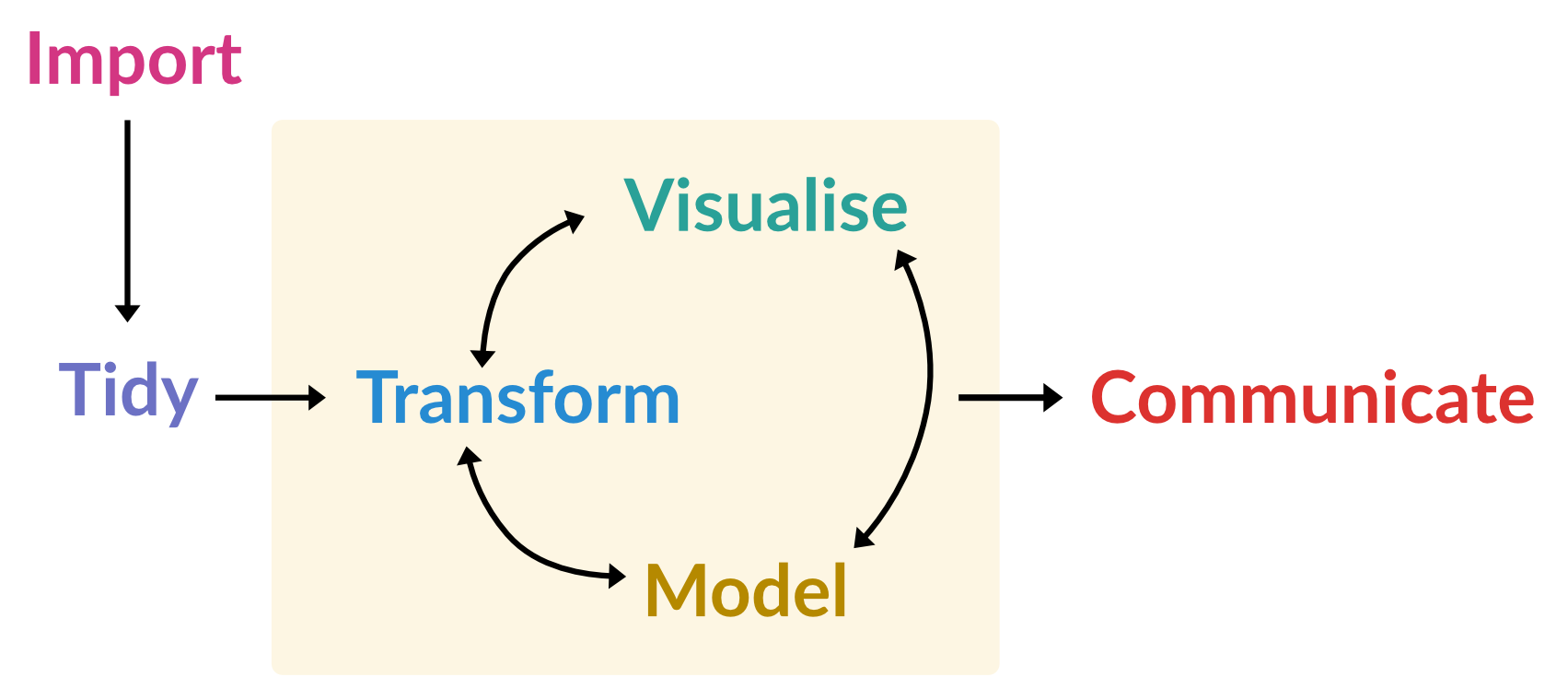
In the second half of the session, we’ll focus on essential data manipulation tasks in R. This will include an introduction to the tidyverse, a powerful collection of packages designed to simplify and enhance data analysis. Through hands-on examples, we’ll cover core steps for working with data, including:

Timetable

Time Topic Slides and practicals
13:00 β€” 13:50 Functions, iteration, and control flow PDF
13:50 β€” 14:40 Practical 1 HTML
14:40 β€” 14:50 Break
14:50 β€” 16:55 Data manipuation in R
Includes three short practicals and breaks
PDF
16:55 β€” 17:00 Wrap up and looking ahead

Practical solutions

This section contains solutions to the reshaping practical at the end of the β€˜Data manipulation’ lecture.

  1. Reshape the fish_encounters dataset to β€˜wide’ format, such that each column represents a different monitoring station.
library(tidyverse)
── Attaching core tidyverse packages ──────────────────────── tidyverse 2.0.0 ──
βœ” dplyr     1.1.4     βœ” readr     2.1.5
βœ” forcats   1.0.1     βœ” stringr   1.5.2
βœ” ggplot2   4.0.0     βœ” tibble    3.3.0
βœ” lubridate 1.9.4     βœ” tidyr     1.3.1
βœ” purrr     1.1.0     
── Conflicts ────────────────────────────────────────── tidyverse_conflicts() ──
βœ– dplyr::filter() masks stats::filter()
βœ– dplyr::lag()    masks stats::lag()
β„Ή Use the conflicted package (<http://conflicted.r-lib.org/>) to force all conflicts to become errors
head(fish_encounters)
# A tibble: 6 Γ— 3
  fish  station  seen
  <fct> <fct>   <int>
1 4842  Release     1
2 4842  I80_1       1
3 4842  Lisbon      1
4 4842  Rstr        1
5 4842  Base_TD     1
6 4842  BCE         1
fish_encounters |>
  pivot_wider(
    names_from = station,
    values_from = seen
  )
# A tibble: 19 Γ— 12
   fish  Release I80_1 Lisbon  Rstr Base_TD   BCE   BCW  BCE2  BCW2   MAE   MAW
   <fct>   <int> <int>  <int> <int>   <int> <int> <int> <int> <int> <int> <int>
 1 4842        1     1      1     1       1     1     1     1     1     1     1
 2 4843        1     1      1     1       1     1     1     1     1     1     1
 3 4844        1     1      1     1       1     1     1     1     1     1     1
 4 4845        1     1      1     1       1    NA    NA    NA    NA    NA    NA
 5 4847        1     1      1    NA      NA    NA    NA    NA    NA    NA    NA
 6 4848        1     1      1     1      NA    NA    NA    NA    NA    NA    NA
 7 4849        1     1     NA    NA      NA    NA    NA    NA    NA    NA    NA
 8 4850        1     1     NA     1       1     1     1    NA    NA    NA    NA
 9 4851        1     1     NA    NA      NA    NA    NA    NA    NA    NA    NA
10 4854        1     1     NA    NA      NA    NA    NA    NA    NA    NA    NA
11 4855        1     1      1     1       1    NA    NA    NA    NA    NA    NA
12 4857        1     1      1     1       1     1     1     1     1    NA    NA
13 4858        1     1      1     1       1     1     1     1     1     1     1
14 4859        1     1      1     1       1    NA    NA    NA    NA    NA    NA
15 4861        1     1      1     1       1     1     1     1     1     1     1
16 4862        1     1      1     1       1     1     1     1     1    NA    NA
17 4863        1     1     NA    NA      NA    NA    NA    NA    NA    NA    NA
18 4864        1     1     NA    NA      NA    NA    NA    NA    NA    NA    NA
19 4865        1     1      1    NA      NA    NA    NA    NA    NA    NA    NA
  1. After reshaping, is this dataset β€˜tidy’? Why?

No. It was already tidy, before reshaping.

  • Before: station and seen in separate columns.
  • After: station stored in the column headers; values in the cells.
  1. Reshape the world_bank_pop dataset to β€˜long’ format, such that it contains three columns: country, indicator, year, and value.
head(world_bank_pop)
# A tibble: 6 Γ— 20
  country indicator       `2000`  `2001`  `2002`  `2003`  `2004`  `2005`  `2006`
  <chr>   <chr>            <dbl>   <dbl>   <dbl>   <dbl>   <dbl>   <dbl>   <dbl>
1 ABW     SP.URB.TOTL     4.16e4 4.20e+4 4.22e+4 4.23e+4 4.23e+4 4.24e+4 4.26e+4
2 ABW     SP.URB.GROW     1.66e0 9.56e-1 4.01e-1 1.97e-1 9.46e-2 1.94e-1 3.67e-1
3 ABW     SP.POP.TOTL     8.91e4 9.07e+4 9.18e+4 9.27e+4 9.35e+4 9.45e+4 9.56e+4
4 ABW     SP.POP.GROW     2.54e0 1.77e+0 1.19e+0 9.97e-1 9.01e-1 1.00e+0 1.18e+0
5 AFE     SP.URB.TOTL     1.16e8 1.20e+8 1.24e+8 1.29e+8 1.34e+8 1.39e+8 1.44e+8
6 AFE     SP.URB.GROW     3.60e0 3.66e+0 3.72e+0 3.71e+0 3.74e+0 3.81e+0 3.81e+0
# β„Ή 11 more variables: `2007` <dbl>, `2008` <dbl>, `2009` <dbl>, `2010` <dbl>,
#   `2011` <dbl>, `2012` <dbl>, `2013` <dbl>, `2014` <dbl>, `2015` <dbl>,
#   `2016` <dbl>, `2017` <dbl>
longer <- world_bank_pop |>
  pivot_longer(
    `2000`:`2017`,
    names_to = "year",
    values_to = "value",
    names_transform = parse_number
  )
  1. Reshape the table2 dataset such that there are separate columns for cases and population.
head(table2)
# A tibble: 6 Γ— 4
  country      year type           count
  <chr>       <dbl> <chr>          <dbl>
1 Afghanistan  1999 cases            745
2 Afghanistan  1999 population  19987071
3 Afghanistan  2000 cases           2666
4 Afghanistan  2000 population  20595360
5 Brazil       1999 cases          37737
6 Brazil       1999 population 172006362
table2 |>
  pivot_wider(names_from = type,
              values_from = count)
# A tibble: 6 Γ— 4
  country      year  cases population
  <chr>       <dbl>  <dbl>      <dbl>
1 Afghanistan  1999    745   19987071
2 Afghanistan  2000   2666   20595360
3 Brazil       1999  37737  172006362
4 Brazil       2000  80488  174504898
5 China        1999 212258 1272915272
6 China        2000 213766 1280428583